Teaching a Machine to Stock ATMs: Deep Reinforcement Learning for Cash Demand Forecasting
Project description
- Primary paper: Zeynalli (2026), Forecasting ATM Cash Demand using Deep Reinforcement Learning
- Domain: Operations management, cash supply chain, time-series forecasting
- Project type: PhD course project (OPIM 613 – Operations and Decision Analytics, Sabancı University)
- Core ideas: DDPG, continuous MDP, online adaptive forecasting, concept drift
Every time you use an ATM, a quiet logistics problem is running in the background. Someone — or more likely some algorithm — decided days ago how much cash to load into that machine. Too much, and the bank is tying up capital in a steel box that earns nothing. Too little, and the machine runs empty, customers leave frustrated, and the bank loses goodwill and fee revenue. Across a network of hundreds or thousands of ATMs spread across a country, even modest improvements in that forecasting accuracy translate into meaningful operational savings.
This project asks a simple but ambitious question: can a self-learning agent trained through trial-and-error do that job better than the statistical models currently in use?
The Problem: Why ATM Cash Is Still Hard to Predict
There is a counterintuitive fact at the heart of this project. Despite the rise of mobile payments and contactless cards, demand for physical cash has not gone away. Economists call this the “cash paradox” — people continue to withdraw cash even as digital alternatives become more convenient. That keeps the forecasting problem commercially alive.
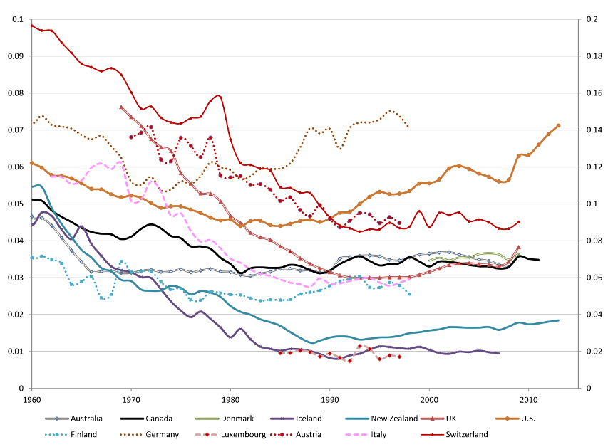 Despite the proliferation of digital payment alternatives, aggregate cash in circulation has continued to grow — the so-called “cash paradox.”
What makes ATM cash demand particularly difficult is its layered structure. A few patterns are predictable: withdrawals tend to spike on Fridays, drop on Tuesdays, and surge around paydays. But beneath those regularities lies a great deal of noise. An ATM near a university behaves very differently from one outside a supermarket. Local events, economic shocks, or a nearby competitor closing can shift demand sharply and without warning.
Traditional forecasting models — ARIMA, regression, and even modern neural networks like LSTM — share a structural weakness: they are trained once on historical data and then frozen. Once deployed, they cannot adapt. If the world changes around them, their predictions get worse and worse until someone manually retrains them. In machine learning, this problem has a name: concept drift.
This project proposes a different approach entirely. Instead of building a model that learns from history and then stops, it builds an agent that never stops learning — one that updates its forecasts continuously based on real-time feedback from the environment.
What the Literature Says
The forecasting literature for ATM cash demand follows a familiar evolution.
Early research used classical time-series models like ARIMA, which decompose demand into trend, seasonality, and noise. These provided interpretable baselines and are still used in practice, but they assume the statistical structure of the data stays constant — an assumption that rarely holds.
As machine learning matured, researchers moved toward more flexible approaches. Neural networks were shown to capture nonlinear demand patterns that linear models missed. Later, deep learning architectures — CNN-LSTM hybrids and “Global” LSTM models trained simultaneously across many ATMs — pushed accuracy further. The best of these methods currently achieve errors roughly half of what a standard ARIMA model produces.
Despite these advances, a core limitation persisted: all of these models are still static. They are trained, validated, and then deployed frozen. Villar and Lengua (2025) reviewed this problem in depth and argued that reinforcement learning offers a structural fix. By treating forecasting as a sequential decision problem, RL agents can update themselves every day as new real demand data arrives. They adapt by design.
RL-based forecasting has already been applied in adjacent domains: electricity load prediction (Zhang et al., 2021), building heat demand (Wang et al., 2022), and ride-hailing volume (Qiao et al., 2023). What had not been done, until this project, was apply it to ATM cash demand.
Framing the Problem as a Decision Process
The central conceptual move in this project is reframing forecasting as a Markov Decision Process (MDP).
In classical forecasting, a model looks at past data and outputs a number. There is no feedback loop — it cannot know in real time whether it was wrong and course-correct.
In an MDP, an agent interacts with an environment over time. Each day, it observes a state (what the world looks like right now), takes an action (makes a forecast), receives a reward (how accurate that forecast was), and moves to a new state. Over thousands of interactions, the agent learns a policy — a strategy for turning observations into forecasts — that maximizes the cumulative reward signal.
The translation is direct:
| MDP Concept | In This Problem |
|---|---|
| State | The last 14 days of cash withdrawals + the day of the week |
| Action | The forecasted demand for tomorrow |
| Reward | A score reflecting how close the forecast was to actual demand |
| Policy | The agent’s learned rule for going from observations to a forecast |
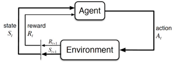 The MDP formulation: the agent observes a state (14-day demand history + day of week), outputs a forecast as its action, receives a reward signal based on accuracy, and transitions to a new state.
One important detail: the action (a cash demand forecast) is a continuous number, not a choice from a menu. This rules out many standard RL algorithms, which assume discrete actions like “buy” or “sell.” It is why this project uses DDPG, an algorithm specifically built for continuous action spaces.
The Reward Signal
The reward function does two things. First, it penalizes raw forecasting error — the bigger the mistake, the lower the reward. Second, it adds a small bonus when the agent correctly predicts the direction of demand change (whether it goes up or down). This bonus was originally proposed by Zhang et al. (2021) as a Reward Incentive Mechanism:
Here is the prediction, is the true demand, and is the size of the directional bonus.
The motivation is practical. Even when exact magnitudes are uncertain, knowing whether demand will be higher or lower tomorrow has real operational value for cash-loading decisions. The reward function is designed to recognize and encourage that.
The Architecture: How DDPG Works
Deep Deterministic Policy Gradient (DDPG) is an actor-critic algorithm. Two neural networks collaborate to learn the forecasting policy.
Actor and Critic
The Actor is the forecaster. It takes the current state — the 14-day demand history plus the day of the week — and outputs a single number: the predicted demand for tomorrow. Structurally, it is a two-layer neural network with 400 and 300 neurons in the hidden layers, using standard deep learning components (Batch Normalization, ReLU activations) to stabilize training.
The Critic is the evaluator. It takes both the current state and the Actor’s forecast as inputs, and outputs a single estimate: how good was that forecast, in terms of expected future rewards? The Critic does not make predictions itself — it tells the Actor how well it is doing.
Training proceeds through a continuous back-and-forth. The Actor produces forecasts, the Critic evaluates them, and both update their weights. The Actor learns to produce forecasts that the Critic rates highly. The Critic learns by comparing its evaluations against what actually happened.
Two Engineering Tricks That Make It Work
Raw actor-critic training can be unstable because the networks are chasing a moving target — as one updates, it changes the basis for the other. DDPG addresses this with two techniques:
Target networks: Each network maintains a slowly-updated shadow copy. During training, the targets for the Critic are computed using these stable copies rather than the main network weights, which are changing rapidly. The shadow copies track the main networks gently: with a soft update rate of .
Experience replay: Each (state, forecast, reward, new state) tuple is stored in a memory buffer. During each training step, a random mini-batch of 32 past experiences is sampled and used for the update. This breaks the strong temporal correlation between consecutive time steps — a necessary condition for stable neural network training.
Two Training Phases
The training procedure mirrors a realistic deployment scenario:
Offline Phase: The agent trains on approximately two years of historical demand data. Day by day, it constructs its state, makes a forecast, observes the actual demand, and stores the experience. This phase stabilizes the policy before the agent encounters live evaluation.
Online Adaptive Phase: During the 56-day test period, the agent does not freeze. Each day, after making its forecast, it observes the true demand and immediately performs a weight update. Unlike any static model, the agent is still learning during the period it is being evaluated. This is the mechanism through which it handles concept drift.
The full set of hyperparameters used is:
| Parameter | Value |
|---|---|
| Look-back window | 14 days |
| State dimension | 15 |
| Actor learning rate | |
| Critic learning rate | |
| Discount factor | 0.90 |
| Soft update rate | 0.005 |
| Batch size | 32 |
| Directional bonus | 0.1 |
Data
The NN5 dataset is a widely-used academic benchmark from a time-series forecasting competition. It contains daily cash withdrawal records from 111 ATMs across the United Kingdom, spanning two years. Withdrawals show clear weekly seasonality — higher toward the end of the week, lower mid-week — and more diffuse monthly patterns around paydays and the start of each month.
Missing values were handled through a hierarchical imputation strategy: gaps are first filled with data from the same day one week prior, then two or three weeks prior, and finally via linear interpolation. All demand values are scaled to the range before training.
Results
The standard error metric used is SMAPE (Symmetric Mean Absolute Percentage Error), the same measure used in the original NN5 competition. A lower SMAPE means more accurate forecasts.
Overall Performance
The DDPG agent achieved a global average SMAPE of 24.64% across all 111 ATMs. This number tells an interesting but incomplete story.
What Worked
The agent outperformed standard statistical baselines decisively:
- Standard ARIMA: 25.91% SMAPE
- Polynomial Regression: 29.73% SMAPE
More notably, on stable, well-behaved ATMs, the results were genuinely impressive. The best-performing case was ATM 22, where the agent achieved a SMAPE of 12.72%. The forecast closely tracked actual demand, capturing both the weekly seasonality and non-linear demand spikes. The continuous online learning — the fact that the agent kept updating during the test period — appears to have been responsible for this accuracy. The agent adapted as the test environment evolved.
What Did Not Work
Against state-of-the-art ensemble and clustering-based methods, the agent fell short:
| Model | Average SMAPE |
|---|---|
| Aggregated SARIMA (literature best) | 11.63% |
| Clustering + GRNN | 18.44% |
| Ensemble (9 models) | 18.95% |
| LSTM | 19.42% |
| DDPG (this study) | 24.64% |
| ARIMA (Standard) | 25.91% |
| Polynomial Regression | 29.73% |
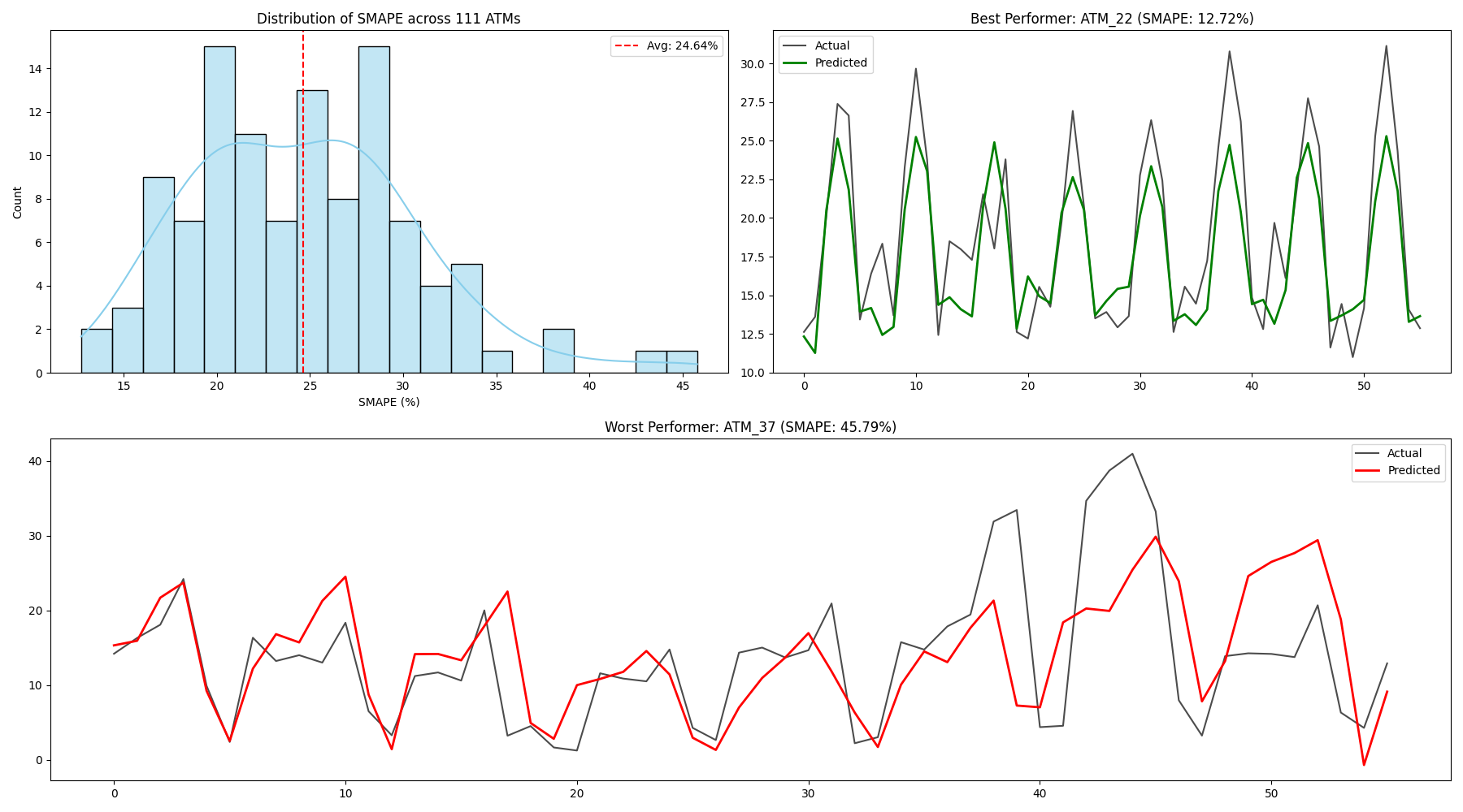 Per-ATM SMAPE distribution across the 111-ATM NN5 dataset. The DDPG agent performs strongly on stable, seasonal machines (e.g. ATM 22: 12.72%) but struggles on volatile, irregular ones (e.g. ATM 37: 45.79%).
The worst case was ATM 37, with a SMAPE of 45.79%. This ATM exhibited irregular, high-magnitude demand spikes without a consistent seasonal structure. Faced with unpredictable patterns, the agent retreated to a conservative policy — essentially making cautious, middle-of-the-road forecasts — which consistently underestimated extreme demand events.
This contrast between ATM 22 and ATM 37 is the most informative result in the study. The DDPG agent is a strong learner when the environment has consistent, learnable patterns. When it does not, the agent’s single shared policy is not flexible enough to adapt across 111 structurally different ATMs simultaneously.
What This Tells Us
The results map out a clear picture of where deep reinforcement learning currently stands in operational forecasting.
RL beats static statistical models. The agent outperforms ARIMA not because it is larger or more complex, but because it keeps learning after deployment. That structural advantage is real and measurable.
RL is not yet a universal forecaster. The best methods in the literature combine multiple specialized models and use clustering to group ATMs by behavioral type. These ensemble approaches hedge their bets by diversifying across many models — something a single neural policy cannot replicate.
The limiting factor is generalization, not learning. The agent’s failure on volatile ATMs is not a failure to learn. It learned extremely well on ATM 22. The failure is that a single policy, trained without ATM-specific tuning, cannot generalize reliably across 111 heterogeneous series.
Two directions emerge naturally from these findings. The first is dynamic model integration: use an RL agent not as the forecaster itself, but as a controller that dynamically assigns weights to a committee of base models — letting it leverage statistical models in stable periods and the learned policy in trend-heavy periods. The second is ATM-specific hyperparameter tuning: rather than using a single hyperparameter configuration for all 111 ATMs, systematically optimize parameters for clusters of ATMs with similar behavioral profiles.
Closing Note
This project sits at the intersection of operations management and machine learning — a PhD course project that attempts to bring a genuinely new methodology to a practical industrial problem.
The honest answer to “can a learning agent replace a hand-crafted ATM forecast?” is: it depends on the ATM. On stable, seasonal machines, it can outperform standard methods while adapting continuously. On volatile, irregular machines, it falls short of specialized ensemble approaches.
That is not a discouraging result. It is an honest map of where reinforcement learning currently stands in real-world operational forecasting — and a precise indication of where the next generation of methods should go.